CALCULATION OF ALERT LEVELS
The purpose of an alert level is to identify significant deviations from a previously acceptable standard of performance. The level should not be set so high that a major increase in the failure rate does not produce an alert, nor so low that the normal distribution of failures results in excessive alerts. The actual setting of the alert level therefore, will normally depend upon the distribution or "scatter" observed in the failure rates of the system under review.
There are several recognized methods of calculating alert levels, any one of which may be used provided that the method chosen is fully defined in the operator's program document. The methods described in the following pages are offered as examples, and many more may be found in any standard text book on statistics.
For purposes of comparison, the first three examples use identical data. It will be seen that the resultant alert levels differ according to the method used, but these small differences are not considered to be of significance. With an effective data display system (see appendix "B") an inappropriately set alert level should be readily apparent.
The symbols used in this appendix have the following conventional meanings:
| x (x bar) | = the mean of a set of data, |
| N | = the number of data, |
| X | = the values of the data, |
| (The Greek capital letter sigma) | = the total of a set of data, |
| (The Greek letter sigma) | = standard deviation, |
| (The Greek letter lambda) | = no of failures, |
| t (The Greek letter Tau) | = time, and |
| (Lambda tau) | = failure rate |
EXAMPLE 1
Pireps -1.3 Mean Alert Level
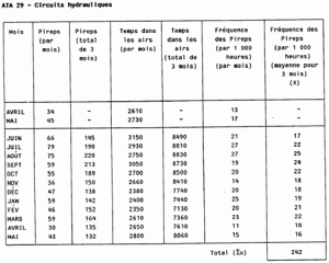
The three month running average Pirep rate per 1,000 hours for each system (or sub-system), as in the table of figure 1 opposite, is averaged over the sample operating period and is known as the mean (x); the mean is multiplied by 1.3 to produce the alert level for the given system.
Although experience has shown this method to be effective with typical fail-ure patterns, it would produce excessive alerts when applied to a system with widely dispersed failure rates, and would not be sufficiently sensitive when applied to data with narrow dispersion.
In the example shown, the alert level (in this case, 26) would be exceeded in the months of July and August.
Appendix A
Figure 1
Number of data in sample (N) = 12
Mean (x) =
x Alert Level = 1.3x N
= 242 = 1.3 x 20
12
= 20 (rounded) = 26
EXAMPLE 2
Pireps -2
alert level (using electronic calculator)
The three month running average Pirep rate per 1,000 hrs for the system (or sub system) is averaged over the sample operating period and is known as the mean (x) as in example 1. The standard devia-tion (the root mean square of the amount by which the data differ from the mean) is calculated as shown, multiplied by 2, and added to the mean to produce the alert level.
Although in the example shown opposite, the resulting alert level is the same as that of the 1.3 x method of example 1, this would not always be the case. A 2
alert is unlike the previous technique in being more respon-sive to the nature of the data, and is particularly suitable for highly scattered data (i.e. data with a high standard deviation).
With a 2
alert, the probability of a spurious alert (one resulting from the scatter of a normal distribution) is approximately 4.5%.
In the example shown, the alert level is obtained by using an electronic calcula-tor having a statistical function. Actual key symbols and sequence may differ according to the model of calculator used.
Step 1:
Select statistical mode: INV (2nd function) MODE (stat or "SD")
Step 2: Clear: INV SAC (clear stats)
Step 3: 17 M+ 22 M+ 25 M+ 24 M+ 22 M+ 18 M+
Enter data: 19 M+ 21 M+ 22 M+ 18 M+ 16 M+
Step 4: key display
Obtain results: Number of data (N) n 12
Total (
x)
x 242
Mean (x) x 20.16666667
Standard Deviation (s)
n 2.763853995
Step 5:
Alert level = 2 x 2.763853995 + 20.16666667 = 25.69437466
rounded to 26
EXAMPLE 3
Pireps -3
alert level
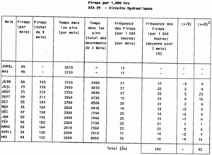
The mean, plus 3 standard deviations as shown in figure 3 opposite. 3
is probably the most common alert level.
A 3
alert is most suited to narrowly scattered data (i.e. data with a small standard deviation), the probability of a spurious alert with this method being 0.3%.
Unlike the previous methods, with the sample data shown, the 3
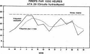
alert level does not produce an alert for the months of July and August. A graphical presentation of the data used in the example is shown below.
Figure 3 - Pireps per 1,000 hrs ATA 29 -Hydraulics
Number of data in sample (N) = 12
Mean (x) =
x Standard Deviation (
) =
(x-x)2
N N
= 242 = 92
12 12
= 20 (rounded) = 7.67
= 2.77
Alert Level = Mean (x) + 3
= 20 + (3 x 2.77)
= 28.31 rounded to 28
EXAMPLE 4
Component unscheduled removals -Poisson method
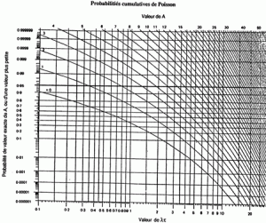
The monitoring of individual components requires either a larger population or a greater experience level than the monitoring of complete systems. The following example is based on 21 months experience, and provides an alert level for use as a 3 month period of comparison. With a large population (either a large number of aircraft or a large number of components per air-craft) the time periods for both experience and comparison could be reduced. The alert level is set at 95% cumulative probability by reference to the chart of Poisson cumulative probabilities on the facing page, as shown in the following two examples:
(a) Component: Autopilot Pitch Amplifier
Number of components per aircraft n = 1
Number of unscheduled removals in past 21 months N = 62
Fleet utilization in past 21 months H = 36840
Component running hours in past 21 months T = (n x H) = 36840
Fleet utilization in current 3 months h = 5895
Component running hours in current 3 months t = (n x h) = 5895
Number of unscheduled removals in current 3 months x = 12
Mean unscheduled removal rate, = N = 0.00168
T
Expected unscheduled removals in current 3 months, = 0.0168 x 5895
= 9.9 rounded to 10 (
Referring to Fig. 4, by entering the graph at t = 10 the intersection with 0.95 (95% probability) gives the maximum acceptable number of unscheduled component removals (A value) for the 3 month period as 15.
By comparing the current value of x = 12 one can see that an "alert" situation does not exist for this component
(b) Component: Temperature Control Valve
Number of components per aircraft n = 3
Number of unscheduled removals in past 21 months N = 31
Fleet utilization in past 21 months H = 36840
Component running hours in past 21 months T = (n x H) = 110520
Fleet utilization in current 3 months t = (n x h) = 17685
Component running hours in current 3 months h = 5895
Number of unscheduled removals in current 3 months x = 9
Mean unscheduled removal rate, = 31 = 0.00028,
110520
Expected number of unscheduled removals in current 3 months = 0.00028 x 17685
= 5.01 rounded to 5 (
From graph acceptable A value = 8.
Current value of x = 9, therefore alert level is exceeded in this case.
Figure 4


